Customer Segmentation at InstaCart
- Ashreet Sangotra
- Aug 24, 2020
- 9 min read


We will be working with InstaCart's popular Market Basket Dataset from Kaggle. Taking a subset of that data and inspiration from some of the kernels, we will be building on those and segmenting our Customers based on purchase activity and products. Links to the dataset and references can be found towards the end of the article.
Pre-Requisites
Even though I will be limiting the code usage on the article, a basic understanding of the following topics is assumed:
Matplotlib for plotting 2-D Data.
Pandas for Data Manipulation
Clustering Algorithms, namely K-Means.
Dimensional Reduction Methods. We will exploring 2 of them - PCA and t-SNE.
Outline
We will divide the project into 6 parts.
Reading and Understanding the Data
Exploring and Visualising Information on products.
Exploring and Visualising Information on Orders.
Clustering by K-Means: Using t-SNE
Clustering by K-Means: Using PCA
Final Conclusions: Understanding Differences between t-SNE and PCA
Reading and Understanding the Data
Our Dataset is compromised of 6 different files. Let's look at their shapes and top 5 rows to get an idea on how we can organise it.


As we can see from above, the datasets can be broadly put into 2 categories:
Online Store layout, categories and products.
Information on Orders and purchases.
A. The first category is made up by 3 files - dept, aisles and product_info.
- The Online Store is split into departments.
- Departments can be further split in aisles
- Aisles can be further split into products.
B. The second Category is made up of order_prior, order_train, order_info.
- order_prior and order_train are datasets with same features.
- They are just different evaluation sets. For out purpose we will focus on order_prior.
- order_info provides further info on order details.
Now that we have some structure to our datasets, let's explore each category.
Exploring and Visualising Products
The first step here is to merge information of all 3 datasets in this category. As we can see, the shape of the merged dataset is the same as our product_info dataset.

Personal Care, Snacks and Pantry are the departments with most number/variety of products the online store has to offer.

These 21 departments are split into 134 Aisles. It will be messy to view all 134 Aisles, so instead we will take a quick look at the top 10 aisles.

The first bar is 'missing', which means 1258 items (products) haven't been assigned or fall under any of our existing departments. In our 'products' dataframe they are assigned an aisle name of 'missing' and aisle_id of 100.
Exploring and Visualising Orders
Our orders_info dataset has 3 million rows and order_prior dataset has 32 million rows in it. Merging these data-frames will make it huge. And it will seriously hinder our computational efficiency. We will reduce the orders_info size by 1/10th and focus on the first 300000 rows.

'orders_info' is made up of 3 evaluation sets - prior, train and test. Since we are clustering the data, and not doing any supervised learning, we will stick with the prior evaluation set. Also it's the only evaluation set that has more than 300000 items (based on our requirement as mentioned earlier).

As seen above, we merge our 'order_prior' and subsetted 'orders_info' datasets. 'order_train' isn't needed anymore since we ruled out the train evaluation set.
We then set the 'order_id' as the index of the updated 'order_prior' data-frame and also drop the column 'eval_set', since it only stores one value now and won't provide any variance for clustering.
We also see that the column 'days_since_prior_order' has 6.43% NaN values. We will fill those values with the mode value.

Now we have a cleaned Dataset. Let's visualise how the orders are distributed across the week and hour of the day.

More orders are placed during the Weekend. For most of the weekdays, more orders are placed in the morning and evening times. Afternoons usually have lesser traffic on weekdays.
Next, we would like to see which products are most ordered. However this would need us to combine 'order_prior' and 'products' into one main data-frame.
That has been done below. Note that the total rows in the data-frame are now 3 million after merging. This number would have been extremely high had we not subsetted the orders earlier.
The merged and updated data-frame 'order_prior' is also the final data-frame we are going to use for clustering later.

Let's see which are the most ordered and most re-ordered products.

There is clear trend between these 2. It confirms to us that products that are more likely to be re-ordered, do end up being the most ordered products in the absolute sense.
It's also interesting to see that the most ordered products are mainly fruits and vegetables.
Now that we have done some basic data cleaning and exploration, let's get on and see how we can cluster this data!
Clustering
We have a lot of data to work with. The main goal is to cluster customers (user_id) into different groups based on some category. We will cluster users base on ordering patterns from each aisle. We have too little departments and too many products. So Aisles are a good in-between category.
Let's first make a cross-table between 'user_id' and 'aisle'.

So we have 19340 customers in total, with their orders distributed across 134 different aisles. Do note that data has been truncated here.
We will run our Clustering algorithm on this data-frame.
The Clustering algorithm we will use is K-Means. However we are going to use 2 different Dimension Reductional Methods to see what kind of varied results we get.
We will reduce the dimensions using T-SNE, run K-Means and form the clusters. And then we will run the same process with PCA.
Clustering by K-Means: Using T-SNE
T-SNE stands for t-distributed Stochastic Neighbour Embedding. It calculates similarities between data points, converts them to joint probabilities, and then tries to minimise the divergence in a low dimensional space. We won't be getting into how exactly t-SNE works. You can find out more from sklearn's documentation here or also have it clearly explained with a StatQuest's video on it. Find that here.
Let's use t-SNE and reduce the dimensions to 2 components. t-SNE takes time to compute, as you can see below.

This is how our data looks on a 2-D scatter plot. We will run K-Means on this.

Before predicting clusters on the above data, lets use the elbow method to decide how many clusters should our K-Means have. We will fit K-Means to our transformed data from above, for cluster values from 1 to 30, and then plot the WCSS (Within-Cluster-Sum of-Squares) score for each cluster value. WCSS measure the variability of observations within a cluster. We want the variability to be as less as possible within a cluster and as high as possible between different clusters.

3 - 7 looks like the range of possible values. We will pick n_clusters = 5 for our purpose.
Let's see how K-Means clusters the data with 5 clusters. We initiate the random_state at 10.

We are gonna take the users from each cluster, and look at the average products ordered by a customer for a given aisle.
The plot below will also give us an overview of the differences between our clusters.

The plots above have a lot of data and would be difficult to read in detail. But that's okay, once we get an overall picture, we will break down different qualities of each cluster further.
Note that the cluster numbers start from 0. Some broad inferences we can make from the graph above are:
Cluster 1 have users buying products from different aisles more uniformly than other clusters.
Cluster 2 have users that buy the most products. The mean values on they axis are quite high. My initial guess is that these would be the most loyal customers. We will verify that below.
There are certain aisles and thus products, that are significant for each cluster.
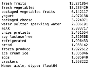
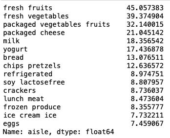
Now let's take a look at the top 15 aisles of each Cluster.
Cluster 0 Cluster 1 Cluster 2


Cluster 3 Cluster 4
- If you look at the top aisles in Cluster 1, we can infer that these are customers who order fast edible and portable items. Since the mean values of this cluster is the least, these are also the customers who shop rarely.
- Cluster 2 is the only cluster with customers shopping in baby food as one of the top aisles. This cluster consists of parents. This could further imply that these customers are more settled, and probably reside in proximity, which makes them a prime target market. This implication is also validated to some extent, given that this cluster has the highest means, thus the loyalest customers (frequent shoppers).
- Cluster 3 are those customers, that don't necessarily prepare food at home, and are more likely to eat outside or grab quick bites through-out the day. We make this inference, since these customers don't shop for fresh vegetables that much, and most of their purchases are ready-to-eat products.
Note: All inferences are based on how we are interpreting the data. To take a definitive action on our inferences, we need to validate these assumptions more thoroughly when in practice.
The common aisles, that are present in each Cluster are - fresh vegetables, fresh fruits, packaged vegetables fruits, yogurt, packaged cheese, milk, chips pretzels and water seltzer sparkling water. Let's see how the orders for these aisles are distributed across different clusters.
% of Orders across top common Aisles for each Cluster

% of Users in each Cluster

We can see from the table users in Cluster 2 make 62.07% of total purchases from these common aisles. Cluster 2, which contains 20.29% of total users is responsible for more than 60% of orders.
Cluster 1 and Cluster 4 represent almost 40% of our customers and yet compromise of only 8-9% of the orders.
Cluster 0 is quite similar to Cluster 2, but less in volume. These could be our future prospects or potential customers.
A visual representation of the distribution can be seen below.

Clustering by K-Means: Using PCA
PCA stands for Principal Component Analysis. You can find out more from sklearn's documentation here.
In this section we will be using PCA for dimension reduction, and apply K-Means to it like above. Do note that the inferences that we get from this will be independent of inferences from t-SNE. However we will try to compare both at the end and see if there are similarities.
Let's use PCA and reduce the dimensions to 6 components. We will then plot a pair-plot to find which component pair to select.

Pair Plots | PCA Components

As we can see from the explained variance ratio, Component 1 is responsible for 48% of the variance and contains the most information.
However from the pair-plots above the combination of Component of (4,5) seem to be best spread for an effective K-Means. We will use components 4 and 5 for our problem.
As before, let's use the elbow method to find out a good estimate for the number of clusters.

4-6 look like decent values for number of clusters. We will go with 4 Clusters this time. Let's look at the clusters we end up with.
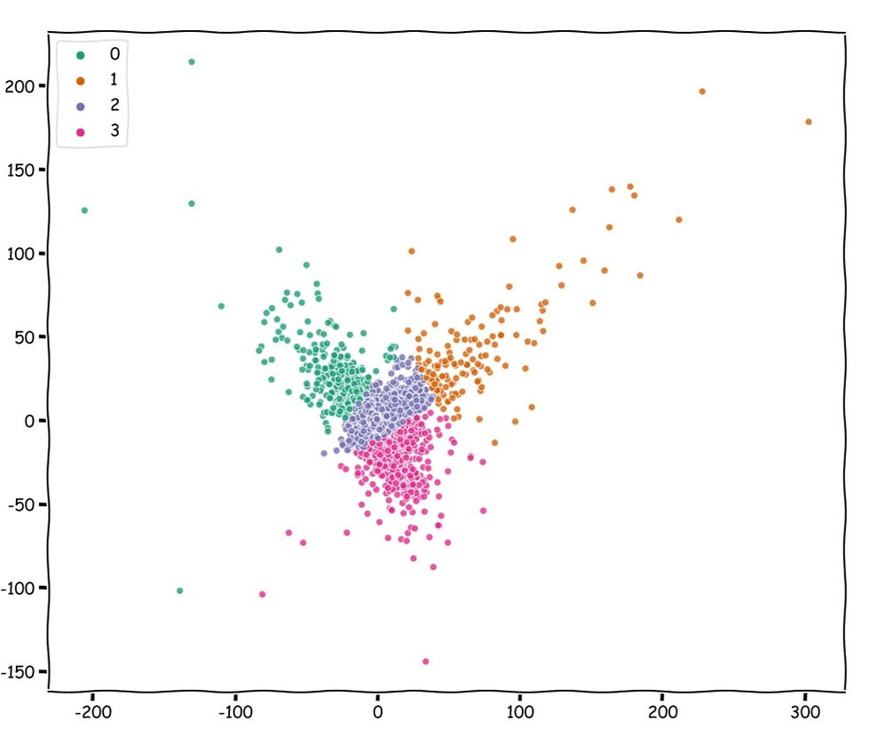
Just like earlier, we are gonna take the users from each cluster, and look at the average products ordered by a customer for a given aisle.

Some broad inferences we can make from the graph above are:
Cluster 0 and 1 have some standout aisles that are not prominent in the remaining clusters.
Cluster 2 have users that buy very few products on an average. The mean values on they axis are quite low.
Just like t-SNE clustering, there are certain aisles and thus products, that are significant in all clusters.
Now let's take a look at the top 15 aisles of each Cluster.
Cluster 0 Cluster 1


Cluster 2 Cluster 3
- Looking at Cluster 1, we see these customers purchase baby products and that too in large quantities.
- With the exception of Cluster 2, the remaining 3 clusters buy lots of products on an average.
Note: All inferences are based on how we are interpreting the data. To take a definitive action on our inferences, we need to validate these assumptions more thoroughly when in practice.
The common aisles, that are present in each Cluster are - fresh vegetables, fresh fruits, packaged vegetables fruits, yogurt, packaged cheese, milk, refrigerated, chips pretzels and soy lactose-free. Let's see how the orders for these aisles are distributed across different clusters.
% of Orders across top common Aisles for each Cluster

% Users in each Cluster

We can see from the table users in Cluster 2 make 67.16% of total purchases from these common aisles. Cluster 2, contains 89.87% of our user base. Our PCA Clustering was able to section out some very specific clusters, but couldn't effectively cluster 90% of our customers. This is mainly due to the loss of information we had when selecting the components. t-SNE does a better job in this regard.
Cluster 0,1 and 3 represent around 10% of our customers and yet compromise of upto 33% of purchases. These customers are regular and loyal.
A visual representation of the distribution can be seen below.

Conclusion
As a general observation, t-SNE clusters are more uniform as they end up capturing most of the variance of the data. PCA fails to do that, but instead provides us with some very specialised clusters.
Both PCA and t-SNE give us different clusters, clustered on different qualities. At the end of the day it depends on wha clusters work best for the business problem.

Comments